PHYSICS OF
THE SPACE ENVIRONMENT
PHYS/EATS
3280
Notes Set
3
The Neutral
Upper Atmosphere
The structure of the upper atmosphere is governed by the basic physical laws of Gravitation, the Ideal Gas Law and Hydrostatic Equilibrium. This leads to a pressure and density variation with altitude of the form shown in Figure 3.1 How can we explain these strong variations in temperature, pressure and density? And how can we predict the temperatures, pressure and air densities at typical spacecraft altitudes ?
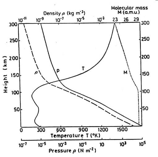
Figure 3.
These questions can be answered
by considering first the fundamental law of hydrostatic
balance or equilibrium.
Hydrostatic equilibrium is the balance between the weight of a gas column and the pressure of the gas. Consider a gas column with density r and of cross-sectional area A as shown in Fig. 3.2.

Fig 3.2
Since pressure is force per unit area
the difference in pressure between the top and bot
P-(P+dP) =grdz
which can be rearranged to give
dP = -rgdz
the equation of hydrostatic balance. By using the ideal gas equation P = rRT/M [where R = 8.314 J mole-1 K-1 is the Universal Gas Constant, r is the density of air in kg m-3, M is mean molecular weight – nominally 0.0289 kg mole-1 - and T is the temperature] we can substitute for r= PM/RT to obtain
dP/P = (-Mg/RT)dz
d lnP = (-Mg/RT)dz
lnP = (-Mg/RT)z + const
or lnP = (-Mg/RT)z + ln P0
or P(z) = P0 exp(-z/H) where H = RT/Mg
H is known as the scale height of the atmosphere and can be locally defined for regions where the temperature is fairly constant. The scale height basically defines how rapidly atmospheric pressure decreases with altitude. It has a value of about 7 km in the very lowest parts of the atmosphere; around 5 km in the middle atmosphere where, as we will see the temperature is very low; but has much larger values towards the top of the atmosphere where the temperatures are very high ~ 55 km at 300 km above the surface.
.
Given that the scale height in the lower atmosphere is only about 7 km, only a small fraction of the total mass of the atmosphere is above about 15 km.
This tenuous gaseous medium that constitutes the upper atmosphere exhibits a considerable range of different characteristics each of which may be used to divide the atmosphere into different regions. These different divisions are summarized in Figure 3.3.

Figure 3.3 The division of the atmosphere in to regions based on various properties
Temperature
Regimes - Division based on temperature structure
The traditional division of the
atmosphere is based on its temperature structure with various 'spheres' where
the temperature gradient is either positive or negative separated by
'pauses'. On the average the temperature
decreases in the troposphere by
about 7 ºC/km up to 10-12 km height where there is a fairly well defined tropopause. The lower stratosphere is at first isothermal but then the temperature
increases as a result of the absorption of solar ultra violet radiation by
ozone. The maximum heating occurs at
about 50 km height and defines the stratopause. Above
this the temperature again decreases to the mesopause which is often rather
ill-defined but can be considered as a region between 80 and 100 km where
the coldest temperatures in the atmosphere occur. Mesopause
temperatures during summer at high latitudes can be as low as 110 K. Above this, in the thermosphere, the
temperature again rises as a result of solar heating at first rapidly but then
more slowly toward the so called exospheric
temperature which, depending on the degree of activity on the sun, can be
anywhere between 800 K at solar minimum and 2500 K at solar maximum. In the thermosphere the heating is mainly due
to photo-dissociation of molecular oxygen and photo-ionization of a
Chemical
Composition Regimes - Division based on composition.
Below about 100 km the composition of the atmosphere can be regarded as constant with the proportions of the main gases being as in Table 3.1
Table 3.1: Composition of the atmosphere at the ground.
Molecule Mass number Volume % Concentration (cm-3)
Nitrogen 28.02 78.1 2.1 x 10¹⁹
Oxygen 32.00 20.9 5.6 x 10¹⁸
Argon 39.96 0.9 2.5 x 10¹⁷
Carbon Dioxide 44.02 0.03 8.9 x 10¹⁵
Neon 20.17 0.002 4.9 x 10¹⁴
Helium 4.00 0.0005 1.4 x 10¹⁴
Water 18.02 variable
The relatively constant
composition is maintained by turbulent mixing and as a result the region can be
designated the turbosphere
or homosphere. Above this the mean distance between the air
molecules is larger than the scale of the eddy motions that mix the homosphere and these can no longer be maintained. Accordingly, the individual component gases
separate according to their molecular weights with the heaviest gravitating
towards the bot
In the homosphere the scale height for all of the main component gases is the same, H=RT/gMav where Mav is the mean molecular weight, while in the heterosphere the concentration of each gas decreases with height in accordance to its own scale height given by H=RT/gMi where Mi is the molecular weight of the individual component in question. The atmosphere is then said to be in diffusive equilibrium with the individual gases establishing their own height variations as defined by there masses and the local temperature. This is of great importance at spacecraft altitudes and is illustrated in Figs. 3.4 and 3.5

Fig 3.4. : The variation of atmospheric composition with height.

Fig 3.5. : More on the variation of atmospheric composition with height.
Variations
in thermospheric composition
In the thermosphere the effects
of molecular diffusion and the lack of turbulent mixing determine the variation
of composition with altitude. Molecular
diffusion becomes rapid because of the increased mean free path between
collisions and the component gases attain their own vertical distributions in
accordance with the hydrostatic law as described above. The action of solar UV radiation to
dissociate molecular oxygen leads to an atmosphere rich in a

Fig. 3.6 : The effect of temperature on exospheric composition. Geopotential heights are given on the left of the diagrams, geometric heights on the right.
Division
based on gaseous escape
Due to the decreasing density of
the atmosphere the mean distance between collisions increases with height and
above about 500 km this distance is so great that a molecule or a![]() is 11.2 km s-1
regardless of the mass of the particle. According to the Maxwell-Boltzmann
velocity distribution only the very lightest molecules and a
is 11.2 km s-1
regardless of the mass of the particle. According to the Maxwell-Boltzmann
velocity distribution only the very lightest molecules and a

Fig. 3.7.
Since hydrostatic equilibrium depends on the gas law and thereby the assumption of a Maxwell-Boltzmann velocity distribution it cannot apply where there is significant gas loss from the atmosphere since the high velocity end of the distribution is being eaten away. Hydrostatic equilibrium should therefore not be assumed above the exobase but the equation is usually used (for want of a better one) to describe the variation of pressure and density with height up to 2000 km.