Initialization 

By combining our understanding of the consumer's preferences and his/her constraints, we can now see how a consumer determines the basket of goods to be consumed.  

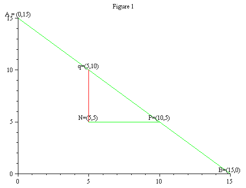
Consider Figure 1, where the budget line is AB.  Clearly, the consumer can reach any indifference curve that is feasible, that is, the consumer can afford a basket of goods that is on or below his budget line. 

The procedure BasknBud plots the relations between the baskets and the budget line. It shows in which direction one moves for the first basket to a second basket and from the first to a third basket. In order to run the procedure one inputs the maximum units of good 1, and the maximum units of good 2 that the consumer is able to buy. This is the 15 in the command line. Next, one inserts, in order, the first basket as [x-coordinate, y-coordinate] followed by the coordinates of the second and third baskets. Thus, to regenerate the figure above, one would execute  

>	BasknBud(15,15,[5,5],[5,10],[10,5]);

 

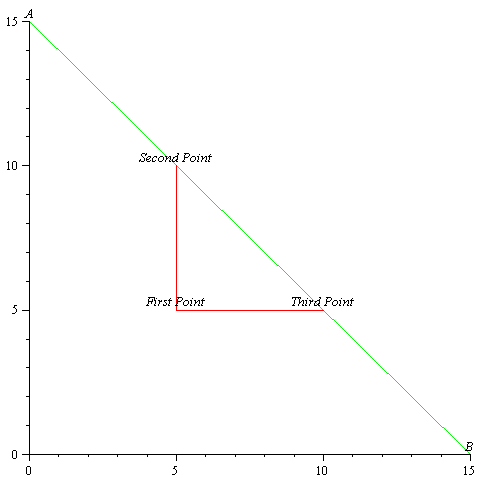To read the value of the coordinate of a point on the graph simply place the mouse at the point and read the coordinate in the upper left windows on the tool bar. The reader is invited to investigate other budget lines and various baskets and their relations. 

Another example one can consider is as follows: 

>	BasknBud(15,10,[5,5],[5,10],[10,5]);

 

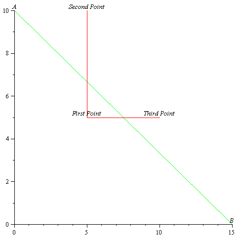Obviously, in this example the second and third points are not feasible. The reader is invited to try other examples. 

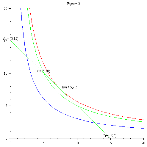
Consider Figure 2. Basket S is on the budget line. Will the consumer choose to consume basket S?  

Once again, the consumer will not. Basket S is on the budget line. This means that the consumer cannot have more of one good without having less of the other. But this particular consumer can do better than S. By moving down and to the right along the budget line, he/she can reach a higher indifference curve. Hence, S is not the consumer's best choice. 

The best choice can be described as the basket of goods which the consumer cannot improve on, given his/her budget constraint. The basket E is the consumer's best choice, because it satisfies this requirement. Any feasible movement away from E puts the consumer on a lower indifference curve, and reduces his/her welfare. 

The point E illustrates an important characteristic which a consumer's best choice usually has: the consumer will generally achieve maximum utility at a point where his/her budget line just touches  (IS TANGENT TO) - does not cross - an indifference curve. We express this by saying that, in equilibrium, the consumer chooses a basket of goods such that the slope of his/her budget line equals the slope of the indifference curve. In terms of our earlier terminology, the consumer maximizes his/her welfare by equating the ratio of the prices of the goods with his/her marginal rate of substitution.  

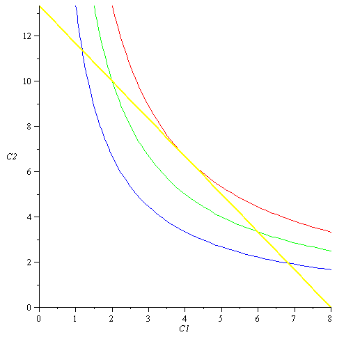
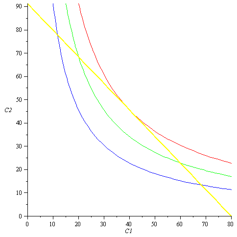
Another way to look at this process is to keep the budget line fixed and plot the indifference curves that cut into the feasible sets. We keep trying a higher indifference curve until we reach the highest one. Note that the higher the curve the higher the welfare. Hence, the highest level of welfare we can reach corresponds to an indifference curve having a unique point in common with the budget line. The procedure below demonstrates this. The input for the procedure is the equation for the budget line and the equation for the indifference curve. The procedure below solves for the optimal basket and illustrates the optimization by graphing the budget line plus three indifference curves. For example, if the budget line is given by and the indifference curves are induced by = the procedure BudnIndiff will generate the required result. 

>	BudnIndif(10*c1+6*c2=80,c1*c2);

 

>

 

The reader can run this procedure for different values of the prices, budget and indifference curve to see the effect on the optimal basket. 

>	BudnIndif(c1+c2/(1.14)=80,c1*c2);

 

>

 

We will return to the mathematical formulation and the systematic solution of the optimal basket.  The procedures BudnIndiff however solve for the optimal basket based on the graphic representation, by recognizing that the optimal basket has two properties. It must be on the budget line and the slope of the budget line at the optimal point (basket) must be equal to the slope of the indifference curve at the optimal point.  

Mathematically if the set such that defines a set of baskets among which the consumer is indifferent, and if this curve is differentiable then the marginal rate of substitution defined above is .  Thinking about as a function of and differentiating both sides of with respect to we  thus have:
 

 
implying that
 

which of course is the result obtained by implicit differentiation. Hence, the short hand notation for the marginal rate of substitution, in terms of , is .  Note that a consequence of our axioms is that both   and    

are positive  as the consumer always prefers more to less. Hence,    is indeed negative which means that, thinking about the indifference curve in the way of, as a function of  , it is a decreasing function. This is consistent with our axioms. 

Therefore, if the budget line is given by ,  the optimal basket is the solution to the two equations stipulated below: 

  and 

The reader is asked in an exercise at the end of the chapter to use the solution approach described above in order to replicate the solution of the procedure for the case: BudnIndif.   

Solving the consumer optimization problem in the manner described above might not work in a case where there is corner solution. In order to formulate this problem and solve it rigorously we must first explain the task of the function and how our assumptions on the family of indifference curves translate to assumptions on – the utility function. This is done in the next section.  

Footnotes